官方网站-首页

　　（来源：OpenCV与AI深度学习）

　　视觉/图像重磅干货，第一时间送达!

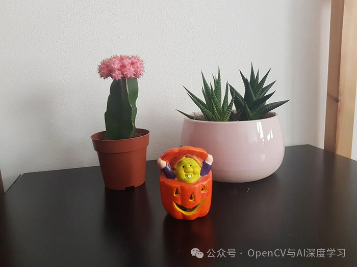
　　    让我们通过一系列智能手机图像来了解小场景的 3D 布局，从而探索 Structure from Motion。选择附近的对象并拍摄相机拍摄的内容有一些重叠的照片。为了获得准确的结果，请使用棋盘格校准您的相机 - 从不同角度拍摄几张照片。此校准步骤为整个过程提供重要信息。

　　1. 引言

　　    运动结构 （SfM） 是一种计算机视觉和摄影测量技术，可重建场景的 3D 结构，并从 2D 图像集合中确定摄像机姿势。通过识别常见特征并求解数学方程式，它将一组图像转换为有凝聚力的 3D 表示，适用于 3D 建模、增强现实和历史景观重建等领域。

　　    以下是求解运动结构 （SfM） 所涉及的步骤的简要分类：

　　2. 特征提取

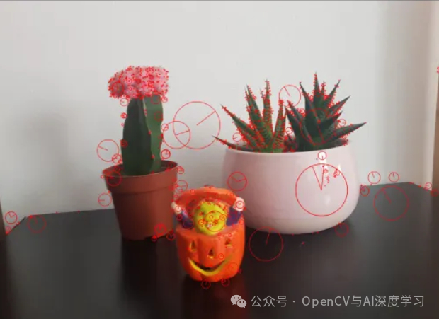
　　    特征提取是从图像中识别和提取独特且可重复的模式或点的过程。这些特征是可以在多个图像之间匹配的关键点，构成了建立对应关系并最终重建 3D 结构的基础。

　　  2.1. SIFT（Scale-Invariant Feature Transform）定义：

　　    SIFT 是由 David Lowe 开发的一种强大的特征提取算法。它对比例、旋转和照明的变化特别可靠，使其成为各种计算机视觉任务的理想选择。

　　void extractFeatures()

{

　　    features_.resize(images_names_.size());

　　    descriptors_.resize(images_names_.size());

　　    feats_colors_.resize(images_names_.size());

　　    for( int i = 0; i

　　    {

　　        std::cout

　　        // Read the image

　　        cv::Mat img = readUndistortedImage(images_names_[i]);

　　        // Create a SIFT detector

　　        cv::Ptr

　　 detector = cv::SiftFeatureDetector::create();

　　        // Create a SIFT descriptor extractor

　　        cv::Mat descriptor;

　　        cv::DescriptorExtractor* extractor = new cv::SiftDescriptorExtractor();

　　        // Detect SIFT features in the image

　　        detector->detect(img, features_[i]);

　　        // Compute SIFT descriptors for the detected features

　　        extractor->compute(img, features_[i], descriptor);

　　        // Store the descriptors for later use

　　        descriptors_[i].push_back(descriptor);

　　        // Extract colors for visualization (optional)

　　        for(int k=0; k

　　            cv::Vec3b color = img.at

　　(features_[i][k].pt);

　　            feats_colors_[i].push_back(color);

　　        }

　　    }

}

　　3. 特征匹配

　　    在运动结构 （SfM） 的上下文中，从多个图像中提取特征后，下一步就是在不同图像中匹配这些特征。此过程旨在建立不同视图中的点之间的对应关系，从而为重建场景的 3D 结构奠定基础。

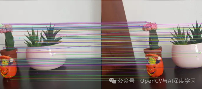
　　    为了对齐不同的图像并在它们的特征之间建立对应关系，我们采用了它们的cv::FlannBasedMatcher接口。该接口利用 Clustering and Search in Multi-Dimensional Spaces 模块，为匹配特征提供了一种快速有效的机制。

　　    为了提高比赛的稳健性，我们实施了距离比率测试。此测试评估给定关键点的两个最接近匹配项之间的距离比率。如果此比率低于某个阈值，则认为匹配是可靠的。这种巧妙的方法有助于区分可能模棱两可的匹配（距离比接近 1）和区分良好的匹配。

　　    此外，我们还为匹配过程引入了一个关键条件。如果认为内部匹配的数量不足（假设小于或等于 10 个匹配），我们将避免在两个图像之间建立匹配。这种实用的检查可以防止包含不可靠的匹配项，从而有助于提高后续重建过程的整体准确性。

　　void exhaustiveMatching()

{

　　    for (int i = 0; i

　　    {

　　        for (int j = i + 1; j

　　        {

　　            std::cout

　　            // Read undistorted images

　　            cv::Mat img1 = readUndistortedImage(images_names_[i]);

　　            cv::Mat img2 = readUndistortedImage(images_names_[j]);

　　            // Create a FLANN-based descriptor matcher

　　            cv::Ptr

　　 matcher = cv::DescriptorMatcher::create(cv::DescriptorMatcher::FLANNBASED);

　　            // Perform K-nearest neighbors matching

　　            std::vector

　　> knn_matches;

　　            matcher->knnMatch(descriptors_[i], descriptors_[j], knn_matches, 2);

　　            // Filter matches using the Lowe's ratio test

　　            const float ratio_thresh = 0.5f;

　　            std::vector

　　 inlier_matches;

　　            for (size_t k = 0; k

　　            {

　　                if (knn_matches[k][0].distance

　　                {

　　                    inlier_matches.push_back(knn_matches[k][0]);

　　                }

　　            }

　　            // Check if the number of inliers is sufficient

　　            if (inlier_matches.size()

　　                continue;

　　            // Set intrinsics matrix and establish matches

　　            intrinsics_matrix_ = new_intrinsics_matrix_;

　　            setMatches(i, j, inlier_matches);

　　        }

　　    }

}

　　4. 三角测量：揭开 3D 的秘密

　　    当我们浏览运动结构 （SFM） 的复杂性时，让我们深入研究三角剖分的过程，这是解开场景 3D 形状的一个基本方面。这个过程通过基本 （E） 和同源 （H） 矩阵展开，每个矩阵在我们的叙述中都发挥着独特的作用。

　　 4.1. 基本矩阵和定位 3D 点：

　　    在充满各种元素的场景中，超越了单纯的平面，Essential 矩阵成为焦点。它隐藏了照相机彼此相对位置的复杂性，为发现 3D 点奠定了基础。利用 OpenCV 的 cv：：findEssentialMat（），我们窥视匹配特征的领域，为 3D 点注入活力。

　　cv::Mat E = cv::findEssentialMat(points0, points1, intrinsics_matrix, cv::RANSAC, 0.99, 1, inlier_mask_E);

　　  4.2. Homography Matrix：揭开平面上的 3D 秘密

　　    但是，当我们的场景主要以平面元素为特色时，Homography 矩阵占据了中心位置。通过使用 cv：：findHomography（），我们简化了流程，促进了这些平面上 3D 点的识别。

　　cv::Mat H = cv::findHomography(points0, points1, inlier_mask_H, cv::RANSAC);

　　int e = cv::sum(inlier_mask_E)[0];

　　        int h = cv::sum(inlier_mask_H)[0];

　　        if( e>h){

　　            cv::recoverPose(E, points0, points1, intrinsics_matrix, init_r_mat,init_t, inlier_mask_E);

　　            seed_found = true;

　　        }

　　    这些矩阵在决策过程中起着至关重要的作用，在后台谨慎运行。输出掩码是一个数字序列，可仔细识别哪些点具有重要性（设置为 1），哪些点具有较低重要性（设置为 0）。在这个关键点和不太关键的点的领域中，出现了一个关键的决定。

　　    我们通过比较关键点的数量来评估 Essential （E） 优于 Homography （H） 的受欢迎程度。如果 Essential （E） 有更多的支持者（更关键的点），我们就会用它来为我们的 3D 世界注入活力，照亮“找到种子”的旗帜。

　　    简而言之，我们的 Structure from Motion （SFM） 之旅就像一场迷人的表演。我们精心选择正确的工具（矩阵），类似于魔法咒语，为我们的场景量身定制，确保我们的 3D 世界完美和谐。

　　5. 揭开和谐的面纱：3D 重建中的 Bundle Adjustment 和 Ceres 求解器

　　    在运动结构 （SfM） 的旅程中，我们介绍了特征提取、匹配和迷人的矩阵世界。现在，让我们来关注一下动态的二重奏：Bundle Adjustment 和 Ceres Solver。

　　 5.1. 光束法调整：精确细化

　　    想象一下为 3D 场景拍摄一系列照片。微小的错误，如轻微的错位，可能会悄悄出现。光束调整功能逐步进入印版，优化相机姿势和 3D 结构，确保更准确的重建。

　　// Bundle Adjustment code snippet

　　void bundleAdjustmentIter(int new_cam_idx)

{

　　    ceres::Solver::Options options;

　　    options.linear_solver_type = ceres::SPARSE_SCHUR;

　　    options.minimizer_progress_to_stdout = true;

　　    options.num_threads = 4;

　　    options.max_num_iterations = 200;

　　    std::vector

　　 bck_parameters;

　　    bool keep_optimize = true;

　　    // Global optimization

　　    while (keep_optimize)

　　    {

　　        bck_parameters = parameters_;

　　        ceres::Problem problem;

　　        // For each observation....

　　        for (int i_obs = 0; i_obs

　　        {

　　            // Check if this observation has been registered

　　            if (pose_optim_iter_[pose_index_[i_obs]] > 0 && pts_optim_iter_[point_index_[i_obs]] > 0)

　　            {

　　                // Extract camera, point, and observation data

　　                double *camera = (parameters_.data()) + (pose_index_[i_obs] * camera_block_size_),

　　                       *point = (parameters_.data()) + (num_poses_ * camera_block_size_ + point_index_[i_obs] * point_block_size_),

　　                       *observation = observations_.data() + (i_obs * 2);

　　                ceres::CostFunction *cost_function =

　　                    ReprojectionError::Create(observation[0], observation[1]);

　　                problem.AddResidualBlock(cost_function,

　　                                         new ceres::CauchyLoss(2 * max_reproj_err_),

　　                                         camera,

　　                                         point);

　　            }

　　        }

　　        ceres::Solver::Summary summary;

　　        Solve(options, &problem, &summary);

　　        // Handle violations and outliers...

　　    }

　　    // Update counts and print pose if a new camera is added

　　    // printPose(new_cam_idx);

}

　　  5.2. Ceres 求解器：优化精度指南

　　    Ceres Solver 是我们的数值优化指南，可与 Bundle Adjustment 无缝协作。它确保对参数进行精确调整，为精确的 3D 重建铺平了道路。

　　// Ceres Solver code snippet (within Bundle Adjustment)

　　ceres::Solver::Summary summary;

　　Solve(options, &problem, &summary);

　　5.3. 残差块和自动微分成本函数：精度

　　    现在，让我们揭开幕后的魔力。Residual Blocks 和 Auto-Differentiable Cost Functions 是无名英雄。残差区组是观测值和预测值之间差值的数学表示。简单来说，它有助于量化需要纠正的 “错误”。

　　struct ReprojectionError

{

　　    ReprojectionError(double observed_x, double observed_y)

　　            : observed_x(observed_x), observed_y(observed_y) {}

　　    template 

　　    bool operator()(const T* const camera,

　　                    const T* const point,

　　                    T* residuals) const {

　　        // camera[0,1,2] are the angle-axis rotation.

　　        T p[3];

　　        ceres::AngleAxisRotatePoint(camera, point, p);

　　        // camera[3,4,5] are the translation.

　　        p[0] += camera[3]; p[1] += camera[4]; p[2] += camera[5];

　　        // Compute final projected point position.

　　        const T predicted_x =  p[0] / p[2];

　　        const T predicted_y =  p[1] / p[2];

　　        // The error is the difference between the predicted and observed position.

　　        residuals[0] = predicted_x - T(observed_x);

　　        residuals[1] = predicted_y - T(observed_y);

　　        return true;

　　    }

　　    // Factory to hide the construction of the CostFunction object from

　　    // the client code.

　　    static ceres::CostFunction* Create(const double observed_x, const double observed_y) {

　　        return (new ceres::AutoDiffCostFunction

(

　　                new ReprojectionError(observed_x, observed_y)));

　　    }

　　    double observed_x;

　　    double observed_y;

};

　　    简而言之，由 Auto-Differentiable Cost Functions 提供支持的 Residual Blocks 量化了我们优化过程中所需的修正。它们将错综复杂的错误转化为数字步骤，Ceres Solver 可以优雅地执行。

　　    下次您目睹令人惊叹的 3D 重建时，请记住幕后大师：光束法平差、Ceres 求解器、残差块和自动微分成本函数。他们是精密的建筑师，使 Structure from Motion 成为视觉奇迹。

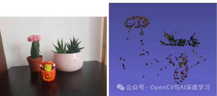
　　    结果直观地显示在点云快照中。利用 MeshLab 渲染和探索生成的 .ply 文件，以获得全面的可视化体验。

　　完整代码：

　　GitHub - sepideh-shamsizadeh/3D_structure_from_motion